Courses
Precalculus
- Affine Coordinate Changes
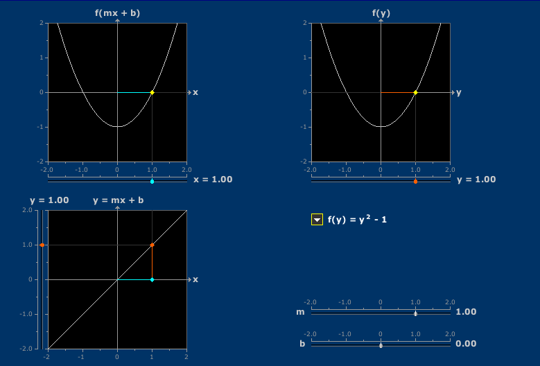
Affine Coordinate Changes
The graph of the function f(mx+b) is related to the graph of f(x) in interesting ways. - Beats
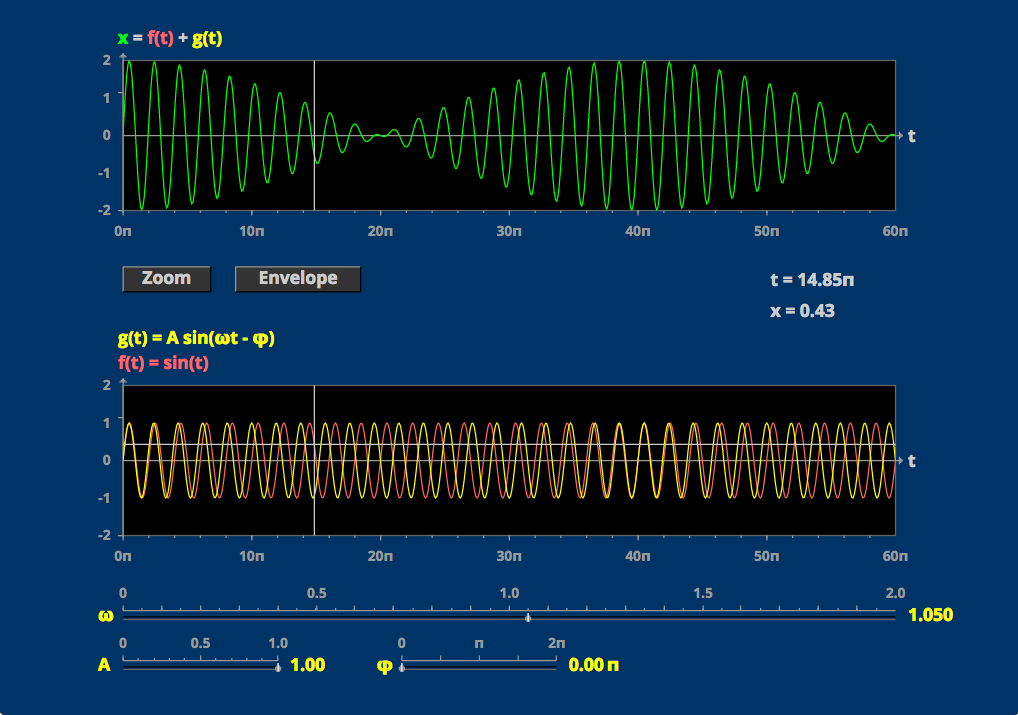
Beats
Beats occur when two sinusoids superimpose. The beat frequency is captured by an envelope. - Beats with Sound
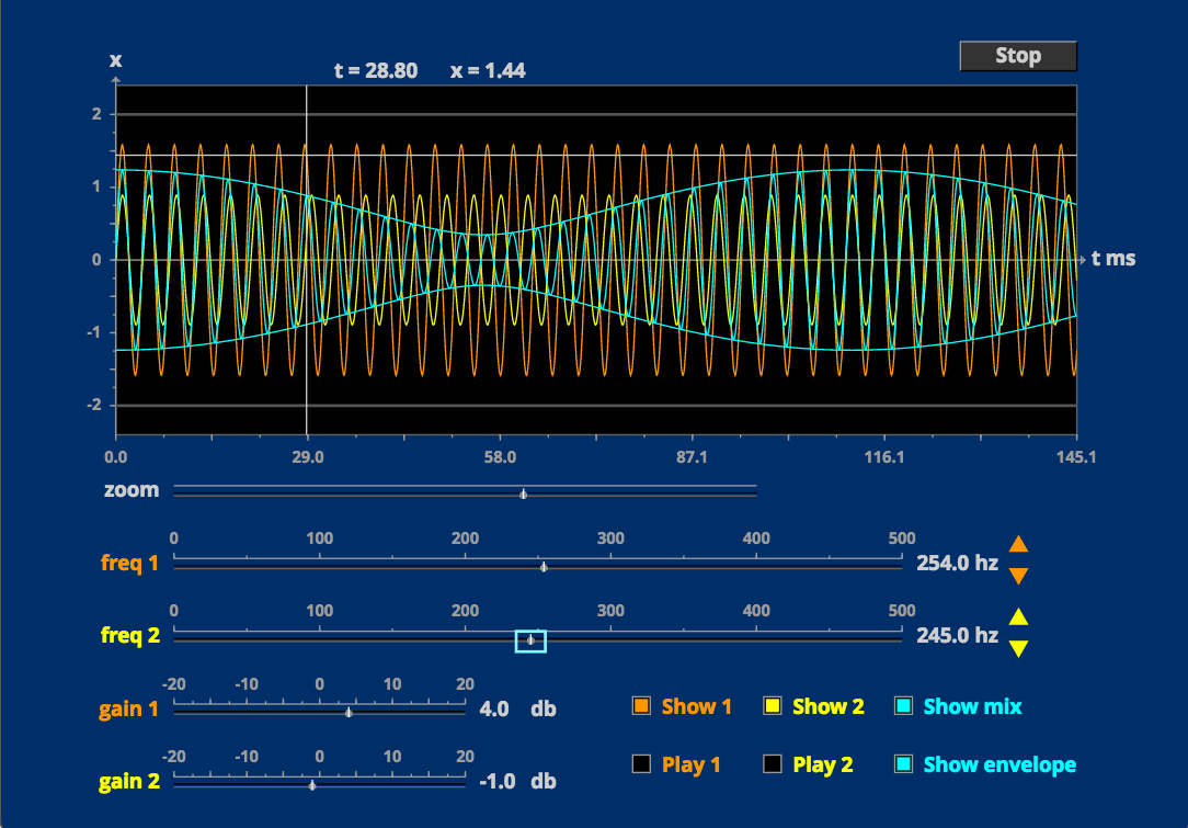
Beats with Sound
Beats with sound, zoom, and units. - Graphing Rational Functions
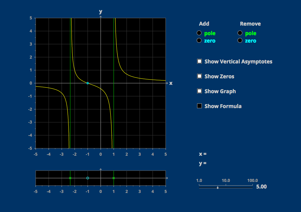
Graphing Rational Functions
The poles and zeros of a rational function let you make a rough sketch of its graph. - Linear Programming
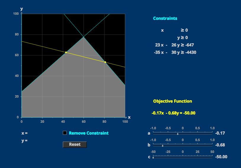
Linear Programming
How do you maximize a linear objective function subject to linear constraints? - Sinusoids
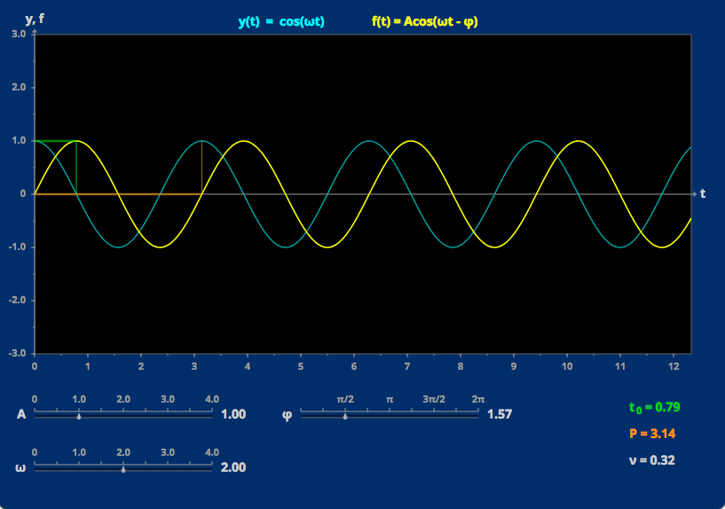
Sinusoids
Any sinusoidal function is a distorted cosine. - Trigonometric Identity
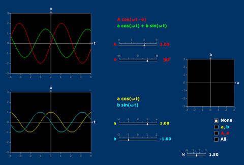
Trigonometric Identity
Any linear combination of cosine and sine (with the same frequency) is again sinusoidal. The amplitude and phase lag of the sum are related to the coefficients of cosine and sine by means of polar coordinates.
Calculus
- Sinusoids
Sinusoids
Any sinusoidal function is a distorted cosine.
1. Differentiaton
- Amplitude and Phase: First Order
Amplitude and Phase: First Order
The tide in a harbor lags behind that of the open ocean, and is controlled by a first order linear equation. Bode and Nyquist plots illustrate the steady state and method of solution. - Creating the Derivative
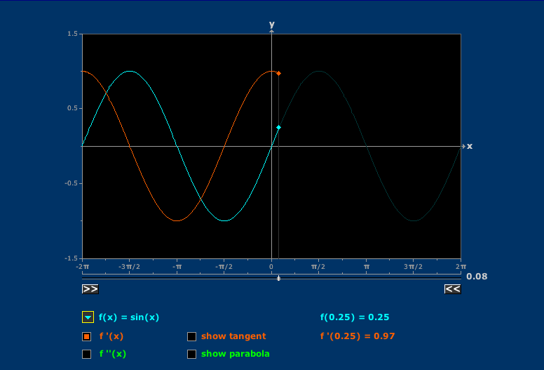
Creating the Derivative
The graphs of f'(x) and of f"(x) reflect interesting features of the graph of f(x). - Hypocycloids
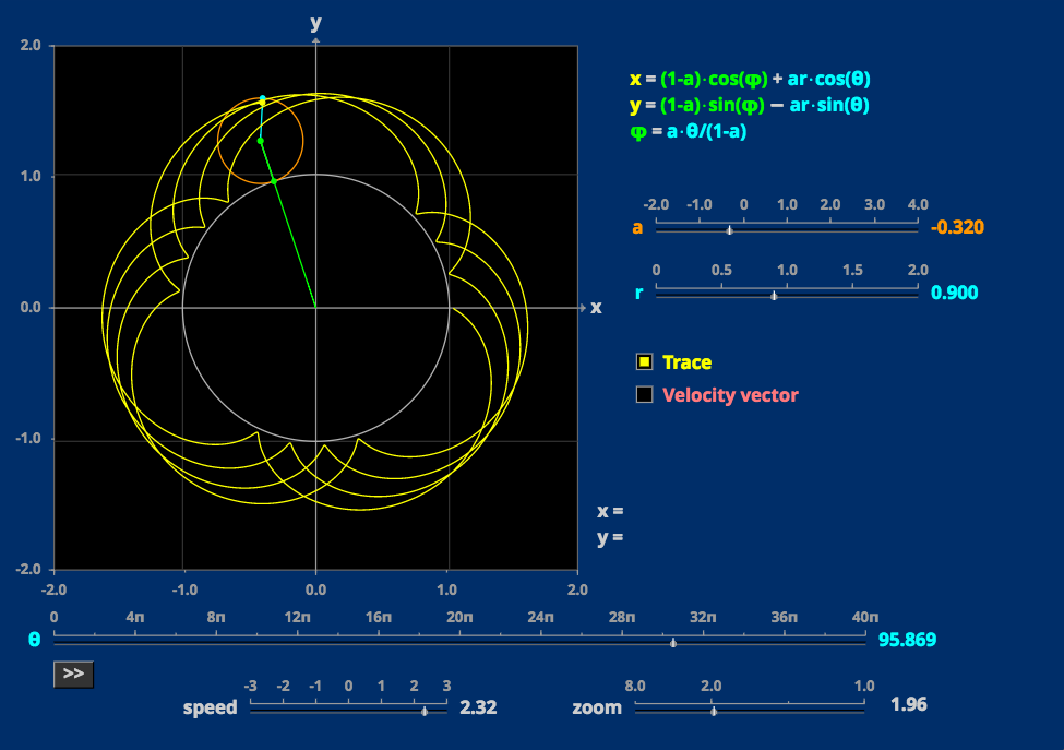
Hypocycloids
Wheels within (or outside of) wheels! - Secant Approximation
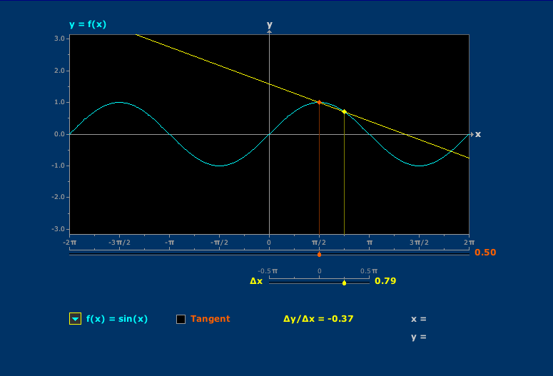
Secant Approximation
Secants converge to tangent lines. - Tangent Approximation
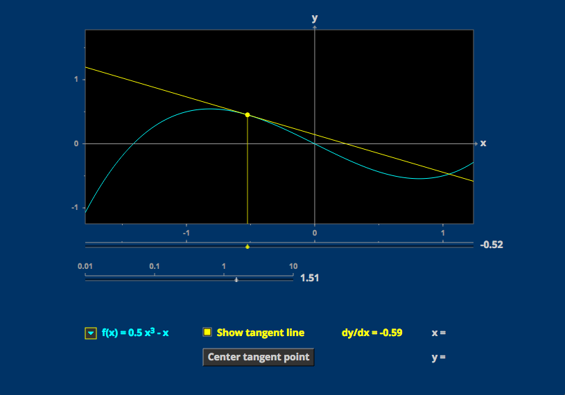
Tangent Approximation
Smooth graphs are close to linear when you blow them up enough.
2. Higher derivatives
- Graph Features
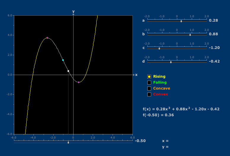
Graph Features
Portions of graphs of cubic polynomials rise, fall, or are convex or concave. - Linearized Trigonometry
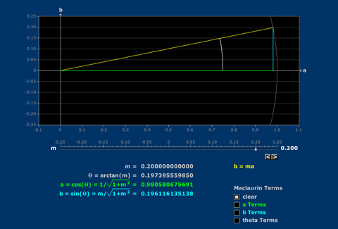
Linearized Trigonometry
For small angles the sine is approximately the angle, but there are higher terms in the Maclauren expansion. - Taylor Polynomials
Taylor Polynomials
Most functions are well approximated near any point by a sequence of polynomials.
3. Integration
- Riemann Sums
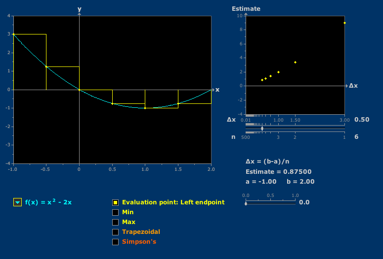
Riemann Sums
An integral can be approximated as a sum in many ways.
4. Vectors and matrices
- Hypocycloids
Hypocycloids
Wheels within (or outside of) wheels! - Matrix Vector
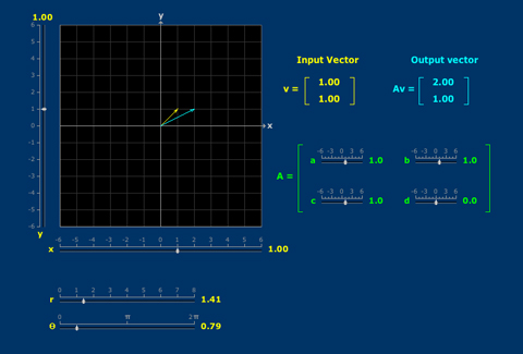
Matrix Vector
The product of a matrix and a vector depends in interesting ways on the entries of each. Eigenvectors represent a coincidence of direction. - Wheel
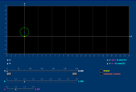
Wheel
A light on a wheel rim traces a curve which may be understood by vector addition.
Differential Equations
1. First order equations
- Ballistic Trajectory
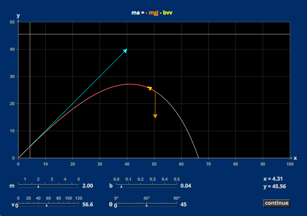
Ballistic Trajectory
A thrown stone responds to the forces of gravity and drag. - Isoclines
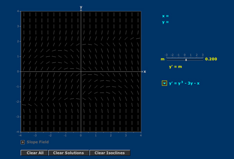
Isoclines
Graphs of solutions of a first order equation can be understood in terms of the slope field and isoclines. - Periodic Box
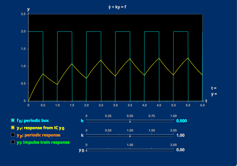
Periodic Box
An impulse train is approximated by "periodic box functions," and the system response to the box function converges to the response to the impulse train as the boxes get narrower. - Solution Targets
Solution Targets
Sometimes solutions converge as time increases, and sometimes they diverge, making the Uniquenss Theorem surprising.
2. More first order equations
- Amplitude and Phase: First Order
Amplitude and Phase: First Order
The tide in a harbor lags behind that of the open ocean, and is controlled by a first order linear equation. Bode and Nyquist plots illustrate the steady state and method of solution. - Euler's Method
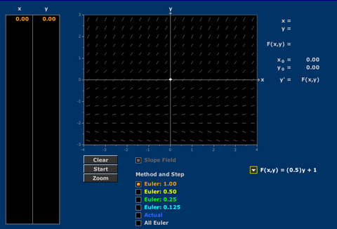
Euler's Method
Given an initial condition and step size, an Euler polygon approximates the solution to a first order differential equation. - Phase Lines
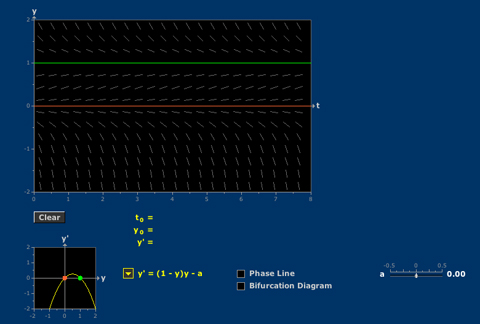
Phase Lines
The nonlinear autonomous equation x' = g(x) can be understood in terms of the graph of g(x) or the phase line. As a parameter in g(x) varies, the critical points on the phase line describe a curve on the bifurcation plane.
3. Complex Numbers
- Complex Arithmetic
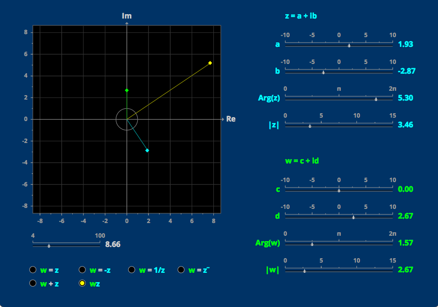
Complex Arithmetic
Complex numbers and operations on them can be visualized on the complex plane. - Complex Exponential
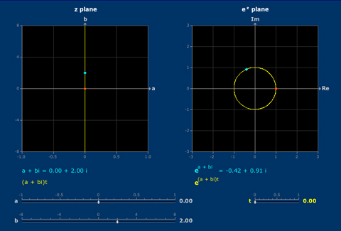
Complex Exponential
The complex exponential function sends straight lines through the origin to spirals. - Complex Roots
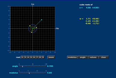
Complex Roots
Any nonzero complex number has n distinct nth roots. - Trigonometric Identity
Trigonometric Identity
Any linear combination of cosine and sine (with the same frequency) is again sinusoidal. The amplitude and phase lag of the sum are related to the coefficients of cosine and sine by means of polar coordinates.
4. Second Order Linear Equations
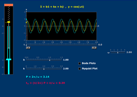
- Amplitude and Phase: Second Order I
Amplitude and Phase: Second Order I
A spring drives sinusoidally a spring/dashpot/mass system. The predictable amplitude and phase lag of the sinusoidal system response can be understood using Bode and Nyquist plots. - Amplitude and Phase: Second Order II
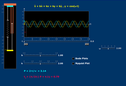
Amplitude and Phase: Second Order II
A dashpot drives sinusoidally a spring/dashpot/mass system. The predictable amplitude and phase lag of the sinusoidal system response can be understood using Bode and Nyquist plots. - Amplitude and Phase: Second Order III
Amplitude and Phase: Second Order III
Both the spring and the dashpot drive sinusoidally a spring/dashpot/mass system. The predictable amplitude and phase lag of the sinusoidal system response can be understood using Bode and Nyquist plots. - Amplitude and Phase: Second Order IV
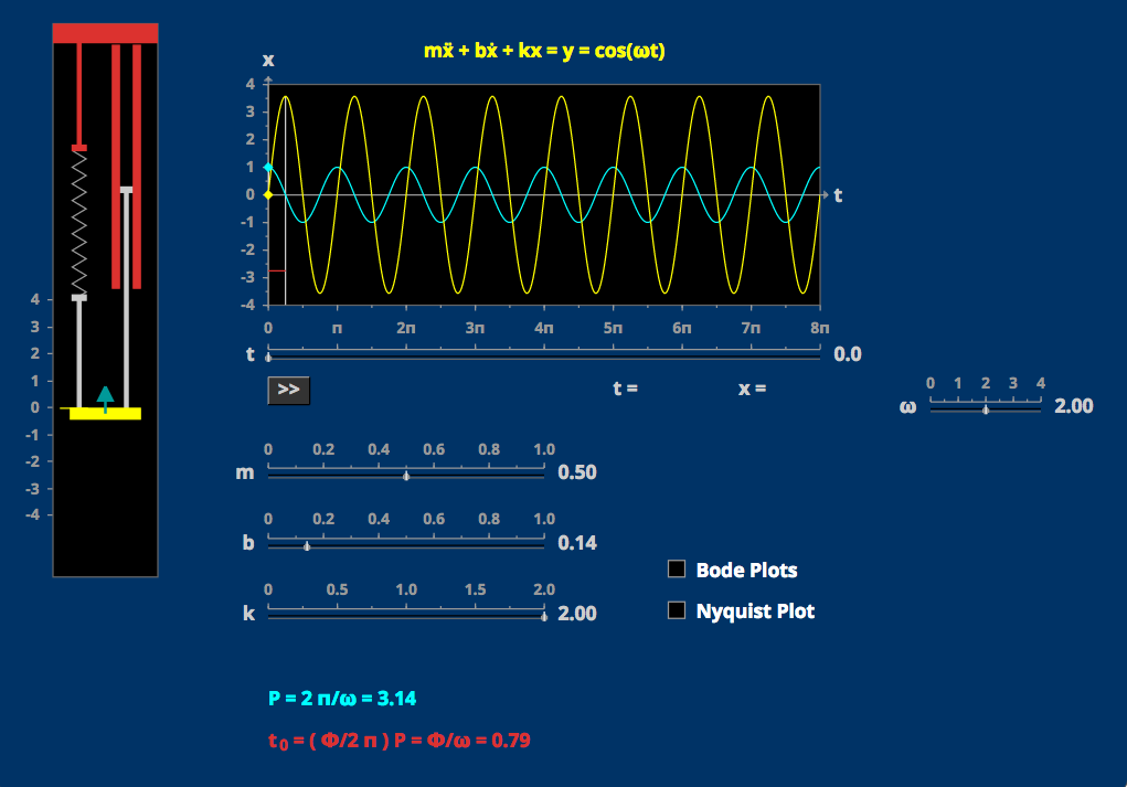
Amplitude and Phase: Second Order IV
A sinusoidally varying force acts directly on the mass in a spring/dashpot/mass system. The predictable amplitude and phase lag of the sinusoidal system response can be understood using Bode and Nyquist plots - Damped Vibrations
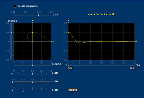
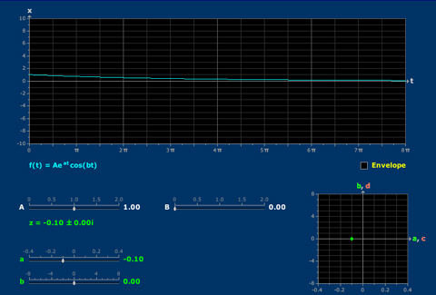
Damped Vibrations
The decay from initial condition to equilibrium of an unforced second order system can be understood using the roots of the characteristic polynomial and the phase diagram. - Forced Damped Vibration
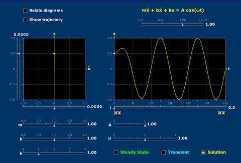
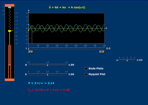
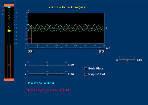
Forced Damped Vibration
The solution to a sinusoidally driven LTI system depends on the initial conditions, and is the sum of a steady state solution and a transient. - Series RLC Circuit
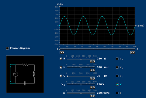
Series RLC Circuit
System responses of a sinusoidally driven RLC circuit can be understood by means of phasors. - Sinusoids
Sinusoids
Any sinusoidal function is a distorted cosine.
5. Convolution, impulse response
- Convolution: Accumulation
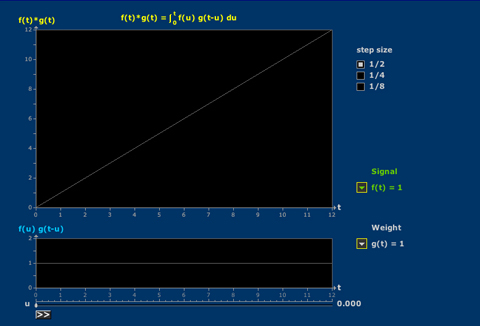
Convolution: Accumulation
The convolution integral is the superposition of unit impulse responses. - Convolution: Flip and Drag
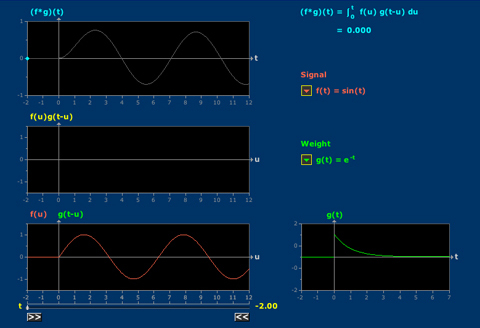
Convolution: Flip and Drag
Convolution at t is computed by integrating the signal weighted by the time reversal of the unit impulse response dragged to start at time t. - Impulse Response: Natural Frequency
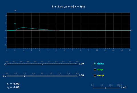
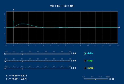
Impulse Response: Natural Frequency
The natural angular frequency and damping ratio determine the system responses to delta, step, and ramp input signals.
6. Fourier series
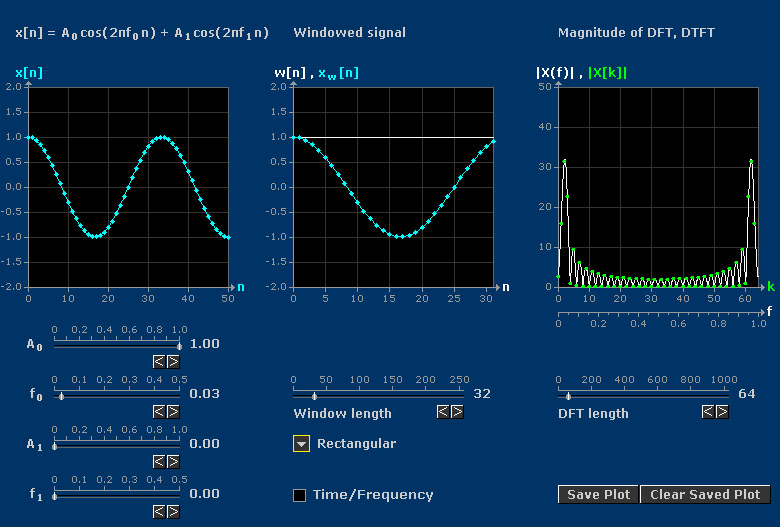
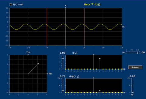
- Fourier Coefficients
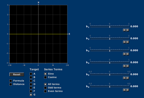
Fourier Coefficients
The initial terms of a Fourier series give the root mean square best fit. Symmetry properties of the target function determine which Fourier modes are needed. - Harmonic Frequency Response: Variable Input Frequency
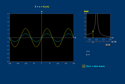
Harmonic Frequency Response: Variable Input Frequency
The periodic frequency response of a harmonic oscillator to a periodic signal depends upon the frequency of the signal. - Harmonic Frequency Response: Variable Natural Frequency
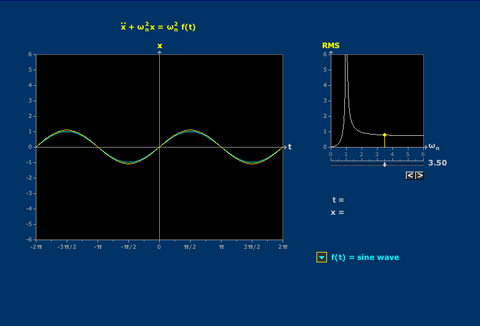
Harmonic Frequency Response: Variable Natural Frequency
The periodic response of a tunable harmonic oscillator to a periodic signal depends upon its natural frequency.
7. Laplace Transform
- Amplitude Response: Pole Diagram
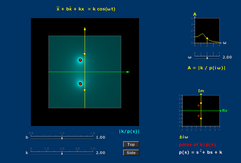
Amplitude Response: Pole Diagram
The exponential response of an LTI system is determined by its transfer function W(s), and roughly by the pole diagram of W(s). The amplitude response or gain is the restriction to the imaginary axis of |W(s)|. - Poles and Vibrations
Poles and Vibrations
A wide range of waveforms occur as the sum of two damped oscillations. The long-term behavior is reflected by the pole diagram of the Laplace transform.
8. Linear systems
- Coupled Oscillators
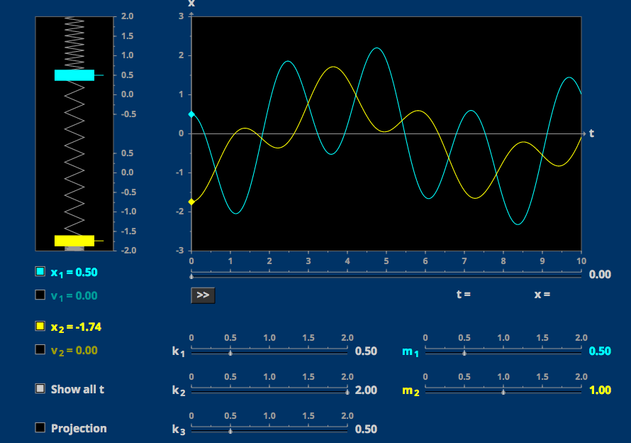
Coupled Oscillators
Two masses and three springs make an interesting dance. For equations, see the Theory page. - Linear Phase Portraits: Cursor Entry
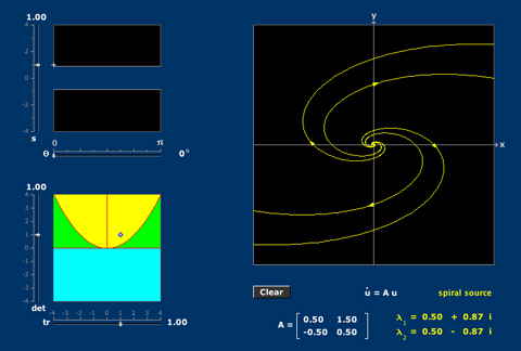
Linear Phase Portraits: Cursor Entry
The phase portrait of a homogeneous linear autonomous system depends mainly upon the trace and determinant of the matrix, but there are two further degrees of freedom. - Linear Phase Portraits: Matrix Entry
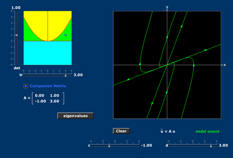
Linear Phase Portraits: Matrix Entry
The type of phase portrait of a homogeneous linear autonomous system -- a companion system for example -- depends on the matrix coefficients via the eigenvalues or equivalently via the trace and determinant. - Matrix Vector
Matrix Vector
The product of a matrix and a vector depends in interesting ways on the entries of each. Eigenvectors represent a coincidence of direction.
9. Partial Differential Equations
- Damped Wave Equation
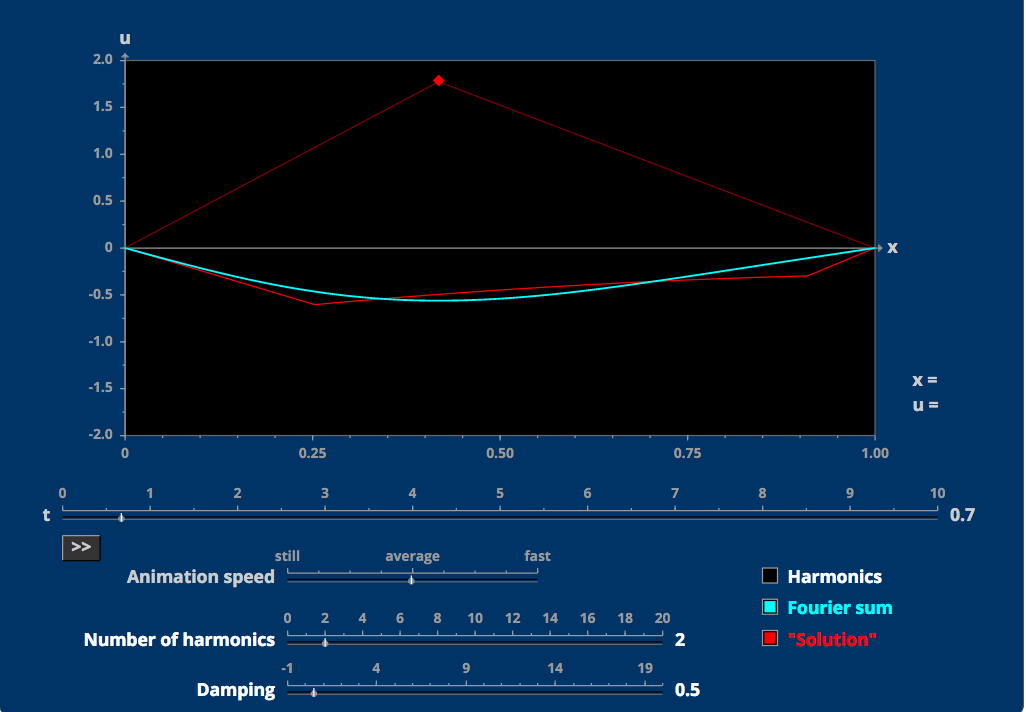
Damped Wave Equation
The vibration of a plucked string dies off because of damping, but can still be understood via Fourier series. - Heat Equation
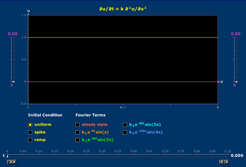
Heat Equation
The evolution of the temperature distribution on an insulated bar can be understood in terms of the Fourier decomposition of the initial condition. - Wave Equation
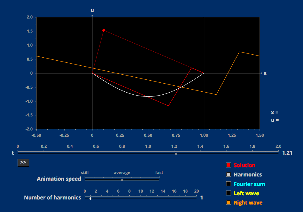
Wave Equation
A plucked string can be analyzed following either Fourier or d'Alembert.
Advanced applications of differential equations
- Amplitude Response: Pole Diagram
Amplitude Response: Pole Diagram
The exponential response of an LTI system is determined by its transfer function W(s), and roughly by the pole diagram of W(s). The amplitude response or gain is the restriction to the imaginary axis of |W(s)|. - Bode and Nyquist Plots
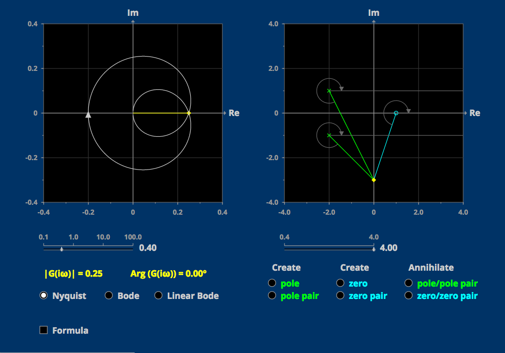
Bode and Nyquist Plots
The system or transfer function determines the frequency response of a system, which can be visualized using Bode Plots and Nyquist Plots. The pole/zero diagram determines the gross structure of the transfer function. - Damping Ratio
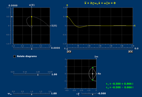
Damping Ratio
The damping ratio and natural frequency of a second order LTI system are determined by the roots of the characteristic polynomial. Initial conditions determine the phase plane trajectory. - Discrete Fourier Transform
Discrete Fourier Transform
- Fourier Coefficients: Complex with Sound
Fourier Coefficients: Complex with Sound
The coefficients in a Fourier series, when it is viewed as a sum of complex exponetials, are best thought of in terms of their magnitude and argument. You can only hear the magnitudes, even though the arguments greatly influence the waveform. - Impulse Response: Spring System
Impulse Response: Spring System
The system parameters determine the system response of a spring system to delta, step, and ramp input signals. - Series RLC Circuit
Series RLC Circuit
System responses of a sinusoidally driven RLC circuit can be understood by means of phasors.
Probability and Statistics
- Beta Distribution
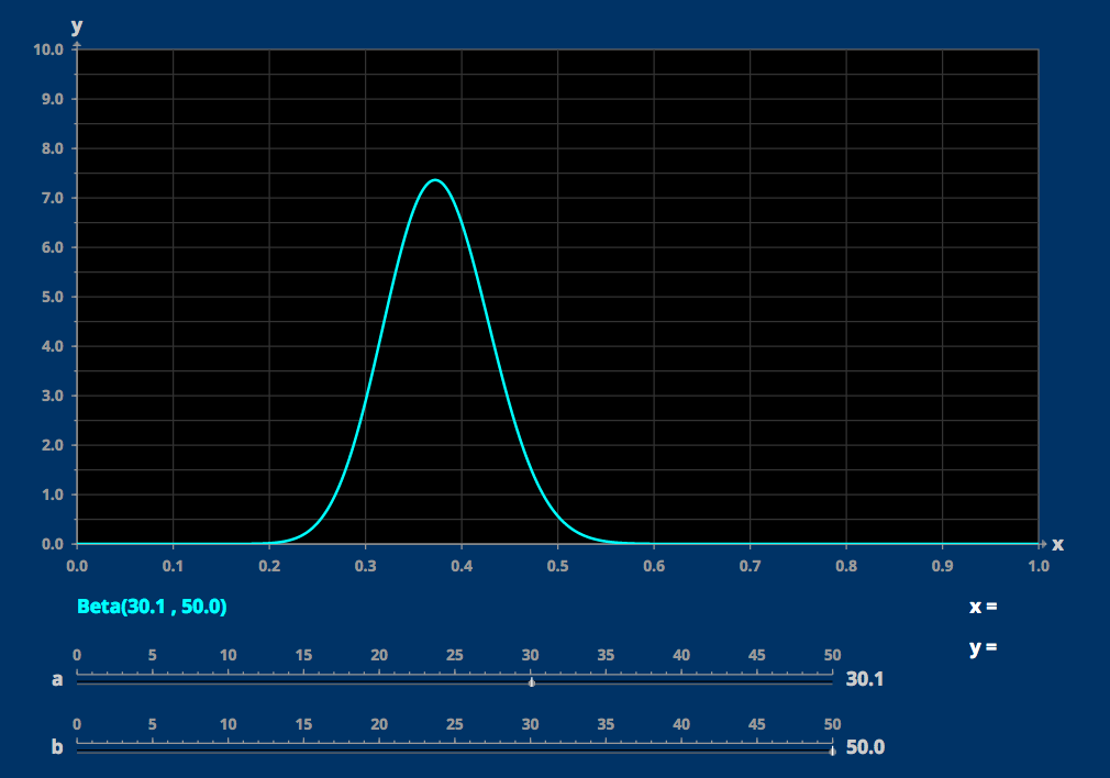
Beta Distribution
The beta-distribution depends on two parameters. - Confidence Intervals
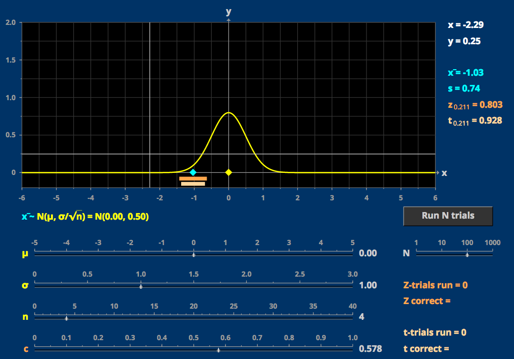
Confidence Intervals
Confidence intervals are range estimates computed from data. - Conjugate Priors
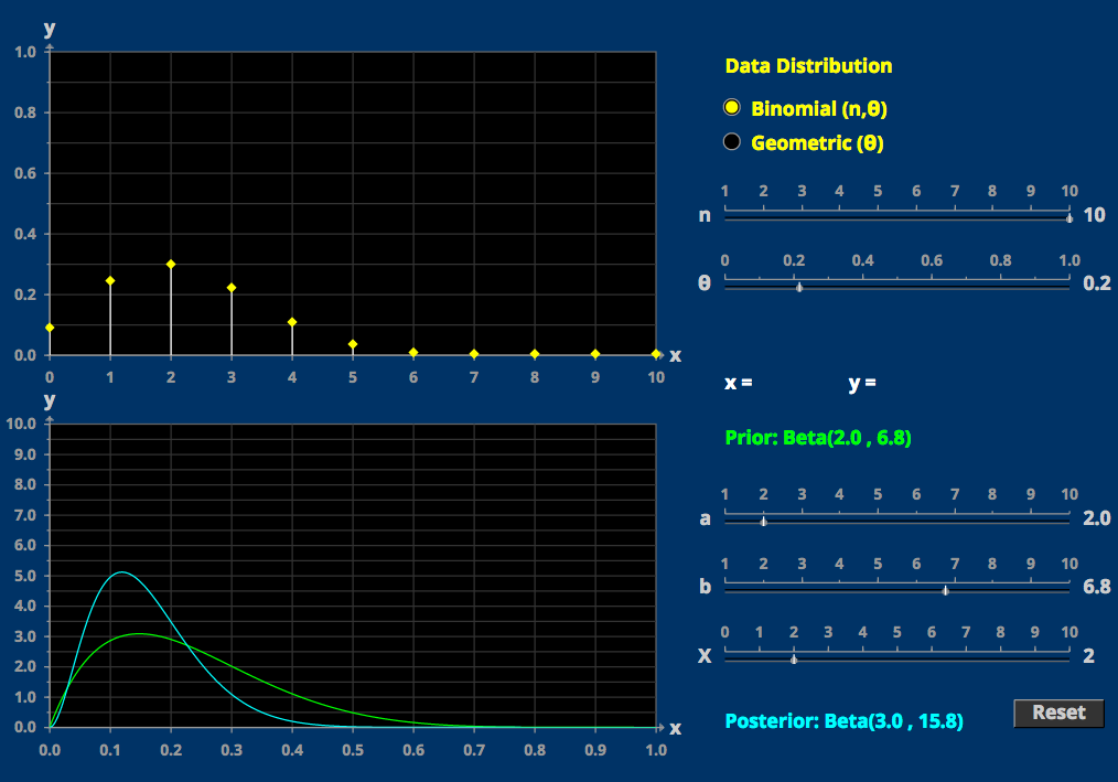
Conjugate Priors
Bayesian updating is easy with conjugate priors. - Linear Regression
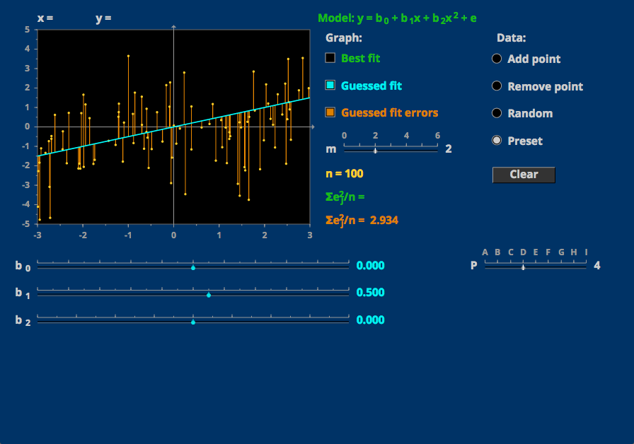
Linear Regression
Data can be fit by a class of functions using least squares. - Probability Distributions
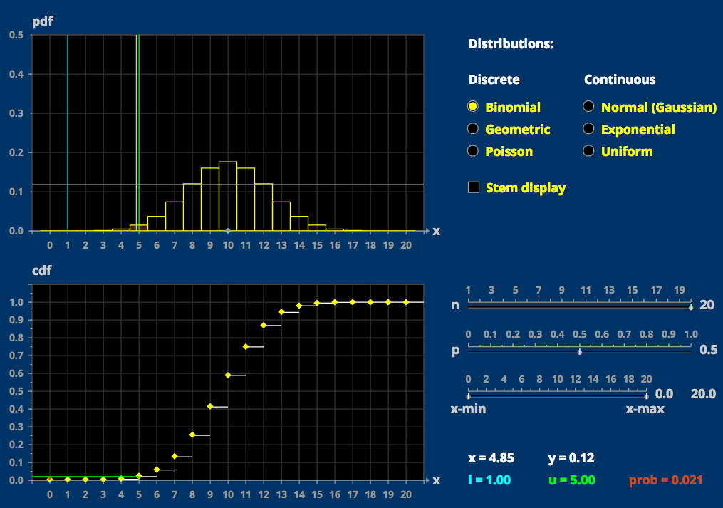
Probability Distributions
Different probability distributions are useful in different situations. - T Distribution
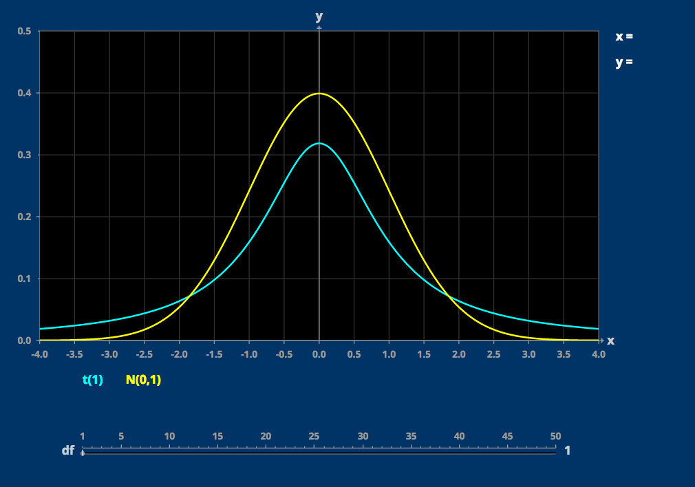
T Distribution
The t distribution depends on one parameter.
